What Is the Optimal Machine Cycle and Why Is It Critical to Industrial Productivity?
The optimal machine cycle represents the technically achievable time interval in which an operation is performed at maximum efficiency, balancing productivity, quality and equipment service life. It is not an isolated theoretical figure; it is a dynamic target that integrates physical, technological and organizational constraints.
Its correct determination is critical because it defines the fundamental heartbeat of any production cell. A poorly calculated cycle generates bottlenecks, excessive idle time or, in the worst case, accelerated deterioration of machinery and quality defects. For the industrial engineer, mastering its calculation is the basis for optimizing any line.
It is vital to distinguish it from other concepts:
- Theoretical Cycle: Nominal time given by the manufacturer, under ideal conditions.
- Observed Cycle: Actual time measured on the shop floor, which includes variability and interferences.
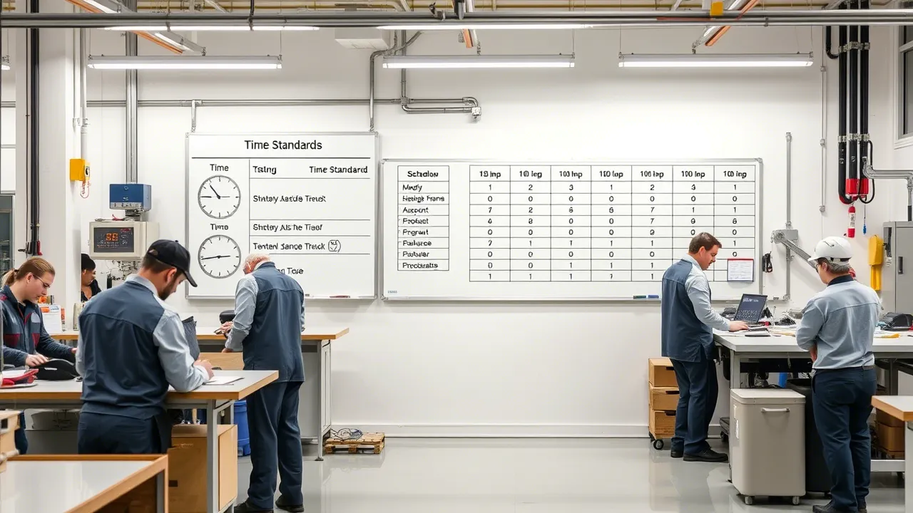
- Standard Cycle: Time calculated after applying allowances for fatigue, rest breaks and personal needs (ILO/OIT standards).
- Optimal Cycle: The efficient convergence between the minimum technological time and the most agile organizational time. It is the benchmark for operational excellence.
Its impact on efficiency is direct and multiplicative. A well-established optimal cycle is the reference against which OEE (Overall Equipment Effectiveness) is measured and line balancing is designed. Tools like Cronometras have greatly simplified the performance of time studies that feed this calculation, making it possible to move from observed data to optimized standards.
Breakdown of Technological Time: The Unshakeable Foundation of the Cycle
Technological time is the backbone of the optimal cycle. It is the component dictated by the laws of physics and process engineering, and it cannot be reduced without changing fundamental parameters of the process itself.
In manufacturing processes, this time breaks down into specific components:
- Active Cutting/Transformation Time: Where the material is modified (machining, laser cutting, forming).
- Solidification/Curing Time: Necessary for the material to acquire its properties (cooling in plastics injection molding, resin curing).
- Chemical Reaction Time: Processes such as anodizing, coatings or surface treatments.
- Energy Transfer Time: Controlled heating or cooling (hardening, baking).
For turning operations, the fundamental formula for the time of a pass is the starting point for any serious calculation:
T = (π · D · L) / (1000 · Vc · f)
Where:
- T: Pass time (min).
- D: Workpiece diameter (mm).
- L: Machining length (mm).
- Vc: Cutting speed (m/min). Depends on the tool material and the workpiece. The factor 1000 converts the speed to mm/min to homogenize the units.
- f: Feed (mm/rev). Tool penetration rate.
This formula calculates the time for a single pass. The depth of cut (ap) does not appear here because it does not affect the time of each individual pass; what it determines is how many passes will be required to remove the excess material. To obtain the total operation time, the pass time is multiplied by the number of passes required:
Number of passes = (Initial diameter − Final diameter) / (2 · ap)
For other chip-removal processes such as milling, the formula changes (π·D is replaced by the tool length and the feed is expressed in mm/tooth or mm/min). The principle is the same: calculate the time from the process geometry and the cutting parameters.
Optimizing technological time means adjusting these parameters within the limits of spindle power, system rigidity and tool life. It is an engineering problem with clear constraints.
Modeling the Man-Machine Interaction to Eliminate Idle Time
In the vast majority of industrial installations, the machine does not work alone. The man-machine interaction is a main source of variability and non-productive time that can pull the real cycle away from the optimal one.
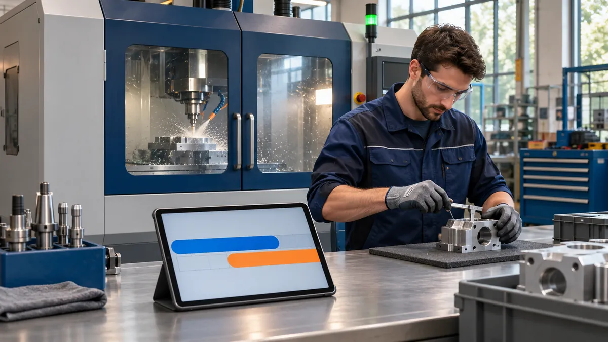
The goal is to model and synchronize activities to minimize interferences. The classic and still irreplaceable tool is the man-machine chart (Man-Machine Chart). This chart allows you to visualize in a synchronized way:
- Operator working time (loading, unloading, measuring, cleaning).
- Machine working time (automatic cycle).
- Times in which one waits for the other (interferences).
When one operator tends several machines, the multiple activity chart is used. The analysis becomes more complex, but the principle is the same: balance the load so that neither the operator nor the machines are idle unnecessarily.
Eliminating idle time requires concrete actions:
- Design of quick-change fixtures (SMED system applied to operations).
- Automation of unloading (collaborative robots, conveyor belts).
- Establishment of parallel inspection routines alongside the automatic cycle.
- Operator training in optimized movement sequences.
Platforms like Induly provide a real-time view of production, making it possible to identify deviations from the planned optimal cycle and analyze root causes, many of which lie in this interaction.
Methodological Evolution: From Classical Time Study to Digital Twins (2025)
Methods and time engineering is not a static discipline. It has evolved by incorporating new technologies while remaining a pillar of productivity.
- First Generation (1940-1970): Classical time study and methods study. It was based on direct observation, the use of stopwatches and the application of allowance tables for fatigue and personal needs, following ILO/OIT principles. It is the foundational basis.
- Second Generation (1970-2000): Predetermined Time Systems (PTS). Systems such as MTM (Methods-Time Measurement) and MOST (Maynard Operation Sequence Technique) made it possible to calculate standard times without the need for time study, breaking the work down into elementary motions with assigned times. They increased accuracy and objectivity.
- Third Generation (2000-2020): Digital integration and simulation. Standard times began to be integrated into planning software (ERP, APS) and process simulation (Tecnomatix, Arena). PLC and SCADA data were used to validate and adjust the calculated standards.
- Fourth Generation (2020-2025): Digital twins, IoT and Machine Learning. Today, digital twins of production cells are created in which cycles are simulated and optimized. IoT sensors capture data in real time, and machine learning algorithms detect micro-stops, anomalies and predict the optimal operating point considering tool wear.
In Spain, the automotive industry leads this adoption, while other sectors advance at uneven rates. Work study is still alive, more powerful than ever as it merges with digital technology. Work sampling, facilitated by applications like WorkSamp, makes it possible to complement continuous studies with random activity analysis, ideal for non-repetitive or highly variable processes.
Tools and Software for Cycle Calculation and Simulation
The choice of tool depends on the budget, the complexity of the process and the plant's level of digital maturity. There is a spectrum of solutions:
- Time Study and Time Measurement: Specialized software such as TiCon or Quetra makes it possible to conduct studies with electronic stopwatches, break down elements, apply performance ratings and allowances, and generate automated standard time reports. They are essential tools for the analyst.
- Predetermined Time Systems (PTS): Specific modules within the above software or dedicated tools for applying MTM-1, MTM-2, MTM-UAS or MOST. They make it possible to calculate times from the drawing or the method description.
- Process Simulation: Platforms such as Tecnomatix (Siemens), Arena or FlexSim make it possible to model the complete production cell, enter cycle times, resources and transport logics, and experiment virtually to find the optimal configuration before implementing it.
- Machine Data Capture (MES/SCADA): Systems such as Siemens Opcenter or SAP ME automatically capture real cycle times from the machines' PLCs, providing the basis for OEE calculation and comparison with the standard.
- Planning and Sequencing (APS): Tools such as Asprova or SAP PP/DS use standard times to sequence work orders and calculate capacities, being major consumers of the data generated by time studies.
The trend is toward integrating these tools into unified platforms that connect the planner, the standard and the actual machine data.
Regulations and Legal Limits in the Design of the Optimal Cycle (Spain/EU)
The optimal cycle cannot be designed on productivity criteria alone. It is heavily constrained by the legal framework on occupational safety and health.
In Spain and the EU, the design of the cycle must respect:
- Machinery Directive 2006/42/EC and its transposition (RD 1644/2008): Ensures that the machine is safe in its operating cycle. It includes requirements for emergency stops, interlocks and protection against mechanical risks.
- Occupational Risk Prevention Act (LPRL) and Specific Regulations: Obligate the assessment of the risks associated with work with machines, including the operator's physical and mental workload. A cycle that imposes an excessive pace or forced repetitive movements may be illegal.
- UNE-EN ISO Standards: Such as ISO 12100 (machine safety) or ISO 11228 (ergonomics, manual handling of loads), which provide technical criteria for safe design.
- Sectoral Agreements and Collective Bargaining Agreements: May establish specific limits on pace, minimum cycle times or mandatory breaks.
The engineer must work hand in hand with the occupational risk prevention technician. The optimal cycle is the one that maximizes productivity within the safe and ergonomic operating space defined by the regulations. Ignoring this is an unacceptable legal and human risk.
Validation and Continuous Improvement through OEE and Data Analysis
The initial calculation of the optimal cycle is only the starting point. Its validation and continuous adjustment are carried out through OEE (Overall Equipment Effectiveness) and production data analysis.
OEE breaks down losses into three categories, directly related to the cycle:
- Availability: Is the machine running when it should be? (Stops due to breakdowns, tool changes).
- Performance: Is it running at the optimal speed (cycle)? (Micro-stops, reduced pace).
- Quality: Does it produce good parts right the first time? (Rejects, rework).
A well-established and respected optimal cycle translates into a high OEE Performance rate. A systematic deviation of the real cycle time from the optimal one is a warning sign that must be investigated.
This is where machine data (via IoT, PLC) is pure gold. They make it possible to:
- Monitor in real time the cycle time part by part.
- Detect deviations and correlate them with variables such as material batch, tool used or operator.
- Feed predictive models that anticipate when the cycle will degrade due to tool wear.
- Verify the impact of implemented improvements (new fixture, cutting parameters).
Continuous improvement (Kaizen) of the optimal cycle thus becomes a data-driven process, not one based on intuition.
Practical Case: Calculating the Optimal Cycle in a CNC Machining Cell
Scenario: Machining of a steel flange on a CNC lathe. Operation: Roughing and finishing of the outside diameter.
Step 1: Calculation of the Time per Pass (T).
- Data: L=100 mm, D=150 mm, Vc=180 m/min (steel with carbide tool), f=0.3 mm/rev (roughing), ap=2 mm.
- Calculation (Roughing): T = (3.1416 × 150 × 100) / (1000 × 180 × 0.3) = 47.124 / 54 = 0.873 min (52.4 s per pass).
- For finishing, with f=0.1 mm/rev, T = 47.124 / 18 = 2.62 min (157 s per pass).
Step 2: Determining the Number of Passes. If the initial diameter of the workpiece is 160 mm and it must be taken down to 150 mm (roughing):
- Radial material to remove: (160 − 150) / 2 = 5 mm per side.
- Passes required: 5 mm / 2 mm (ap) = 3 passes (rounding up to the next integer).
- Total roughing time: 3 × 52.4 = 157.2 s (2.62 min).
Step 3: Man-Machine Analysis. A chart is prepared. The automatic cycle of each roughing pass lasts 52.4 s. The operator needs 18 seg to remove the previous workpiece and mount the new one on the chuck (only at the start of the complete cycle).
- Interference: The machine waits 18 seg before the first pass, but subsequent passes are automatic. The operator can use that time to inspect the previous workpiece.
- Optimization: Implement a quick-change chuck (reduces mounting to 12 sec) and use the automatic cycle time to carry out the dimensional inspection of the previous workpiece in parallel.
Step 3: Determining the Optimal Cycle. Adding the technological time, the loading/effective times and the minimum legal allowances (e.g., 5% for personal needs), a preliminary standard cycle is obtained. This is validated in actual production over one week, measuring the performance OEE.
Step 4: Validation and Adjustment. The MES data show a performance of 92% relative to the preliminary standard. The micro-stop analysis reveals that chip control causes occasional stops of 2-3 seconds. The CNC program is adjusted (chip-breaking parameters) and the optimal cycle is recalculated, improving performance to 97%.
Conclusion: The optimal cycle is not a fixed number, but a living target that is refined with data and analysis.
Frequently Asked Questions (FAQ)
Is classical time study still valid in 2025? Yes, and very much so. It remains the most direct and reliable method for establishing initial standards, especially in manual or assembly processes. Technology has enhanced it: electronic stopwatches connect to software that eliminates calculation errors and generates automatic reports. It is the foundation on which more complex systems are built.
How are MTM or MOST applied to a machine operation? Predetermined systems do not calculate the machine's technological time (that comes from the physics of the process). They are applied to calculate the handling, loading, unloading, checking and transport times performed by the operator or a robot around the machine. The operator's motion sequence is modeled to synchronize it perfectly with the automatic cycle.
What variability is acceptable in cycle time? It depends on the process. In CNC machining, very low variability is expected (<2%). In manual or assembly processes, it can be higher (5-10%). The key is to measure the variability (standard deviation) and establish control limits. Excessive variability indicates an unstable method or lack of control over the process parameters.
Is OEE the same as the optimal cycle? No. OEE is an outcome metric that measures the overall efficiency of an equipment unit. The optimal cycle is a design input. A poorly calculated optimal cycle will make the performance OEE low. A good optimal cycle, well executed, is a necessary (though not sufficient) condition for a high OEE.
How does safety legislation affect cycle calculation? The regulations establish insurmountable limits. For example, if to achieve a theoretical cycle the operator must perform movements that exceed the recommended ergonomic limits (e.g., frequency of lifting loads), that cycle is not valid. The legal optimal cycle is the most productive one within the safe operating space defined by the law.
Resources and Tools
To go deeper into these techniques and find solutions for your plant, we recommend the following resources:
- ASETEMYT Directory: Your database of suppliers and consultants specializing in industrial time study, methods engineering and productivity.
- ASETEMYT Blog: Technical articles, case studies and trend analysis in industrial productivity.
- Production Control Software Induly: To capture actual times, manage stops and calculate OEE in real time.
- Work Sampling Study Application WorkSamp: Conduct Work Sampling studies quickly and accurately.
- Do you offer services in this field? Add your company to the directory and connect with potential clients.
Don't want to do it yourself? We do it for you from €800
If you prefer to outsource it, Cronometras delivers a complete time and motion study from a single video: elemental breakdown, OIT/TAL fatigue allowances, standard time with tolerances, and a report in PDF + Excel + JSON ready to present to management.