Introduction: When the Stopwatch Is Not Enough
Imagine that you carry out a time study on an assembly line. You take 30 time study readings of the same element and obtain a mean of 45 seconds. Pleased, you set the standard time and go home. The next day, the supervisor calls you: the line is producing 18% below expectations.
What happened? The answer lies in variability. That mean of 45 seconds was hiding a standard deviation of 12 seconds, with values ranging from 28 to 74 seconds. The mean alone does not tell the whole story. Statistical Process Control (SPC) applied to industrial time study exists precisely to solve this problem: to understand, measure and control variability before it controls your results.
In this article we will explore how the classic statistical tools of SPC —histograms, control charts, capability analysis— are applied directly to time study, helping you distinguish between the natural variation of the process and the anomalies that require intervention.
Why Does Variability Matter in a Time Study?
Variability in cycle times can be due to a multitude of factors: operator fatigue, skill differences, material variations, micro machine stoppages, environmental fluctuations or simply the randomness inherent in any human activity.
When we ignore variability, we make two serious mistakes:
Underestimation of standard time: if we use the simple arithmetic mean without considering the appropriate allowances, the standard will be too tight, generating pressure on the operators, stress and potential quality problems.
Overestimation of standard time: if we add excessive slack out of fear of variability, we inflate labor costs and lose competitiveness.
SPC gives us an objective framework for making these decisions with data, not with intuitions.
Fundamental Statistical Concepts for the Time Study Analyst
Before getting into the tools, let us review the key concepts:
Arithmetic Mean ($\bar{x}$)
It is the average value of the observations:
Where is each individual observation and is the total number of observations.
Standard Deviation ($s$)
It measures the dispersion of the data with respect to the mean:
A high standard deviation indicates that the times are very irregular; a low one, that the process is consistent.
Coefficient of Variation ($CV$)
It expresses the standard deviation as a percentage of the mean:
It is especially useful for comparing variability between elements of different duration. A above 20-25% usually indicates that the work method is not standardized enough.
Confidence Interval for the Mean
It tells us the range within which the true population mean lies at a given confidence level (usually 95%):
Where is the critical value of the Student t distribution with degrees of freedom.
Calculation of the Number of Observations Required
One of the most practical uses of statistics in time study is to determine how many observations we need. The classic formula based on the maximum allowable error is:
Where:
- is the critical value of the normal distribution (1.96 for 95% confidence)
- is the estimated standard deviation from a pilot sample
- is the maximum allowable error (for example, ±5% of the mean)
Practical example: After a pilot sample of 15 observations of an assembly element, we obtain seconds and seconds. We want a maximum error of ±3% of the mean with 95% confidence:
We would need approximately 187 observations. If this number is greater than the pilot sample, we must continue collecting data.
Control Charts Applied to Time Study
Control charts are the central tool of SPC. For time study, we mainly use two types:
Mean Chart ($\bar{x}$)
It monitors the central tendency of the process. Its control limits are calculated as:
Where is a constant that depends on the subgroup size (for , A_2 = 0.577$) and $\bar{R} is the average range.
Range Chart ($R$)
It monitors variability. Its limits:
Where and are tabulated constants (for : , $D_4=2.114$).
Interpretation: A point outside the control limits indicates a special cause of variation (change of operator, breakdown, defective batch). A run of 7 consecutive points on the same side of the center line suggests a process shift (tool wear, progressive fatigue).
Practical Construction with CronometrasApp
To build these charts, we organize the data into rational subgroups. For example, if we time 5 cycles every hour during an 8-hour shift, we will have 8 subgroups of size 5:
| Hour | Cycle 1 | Cycle 2 | Cycle 3 | Cycle 4 | Cycle 5 | ||
|---|---|---|---|---|---|---|---|
| 08:00 | 44 | 47 | 43 | 48 | 45 | 45.4 | 5 |
| 09:00 | 46 | 44 | 47 | 45 | 43 | 45.0 | 4 |
| ... | ... | ... | ... | ... | ... | ... | ... |
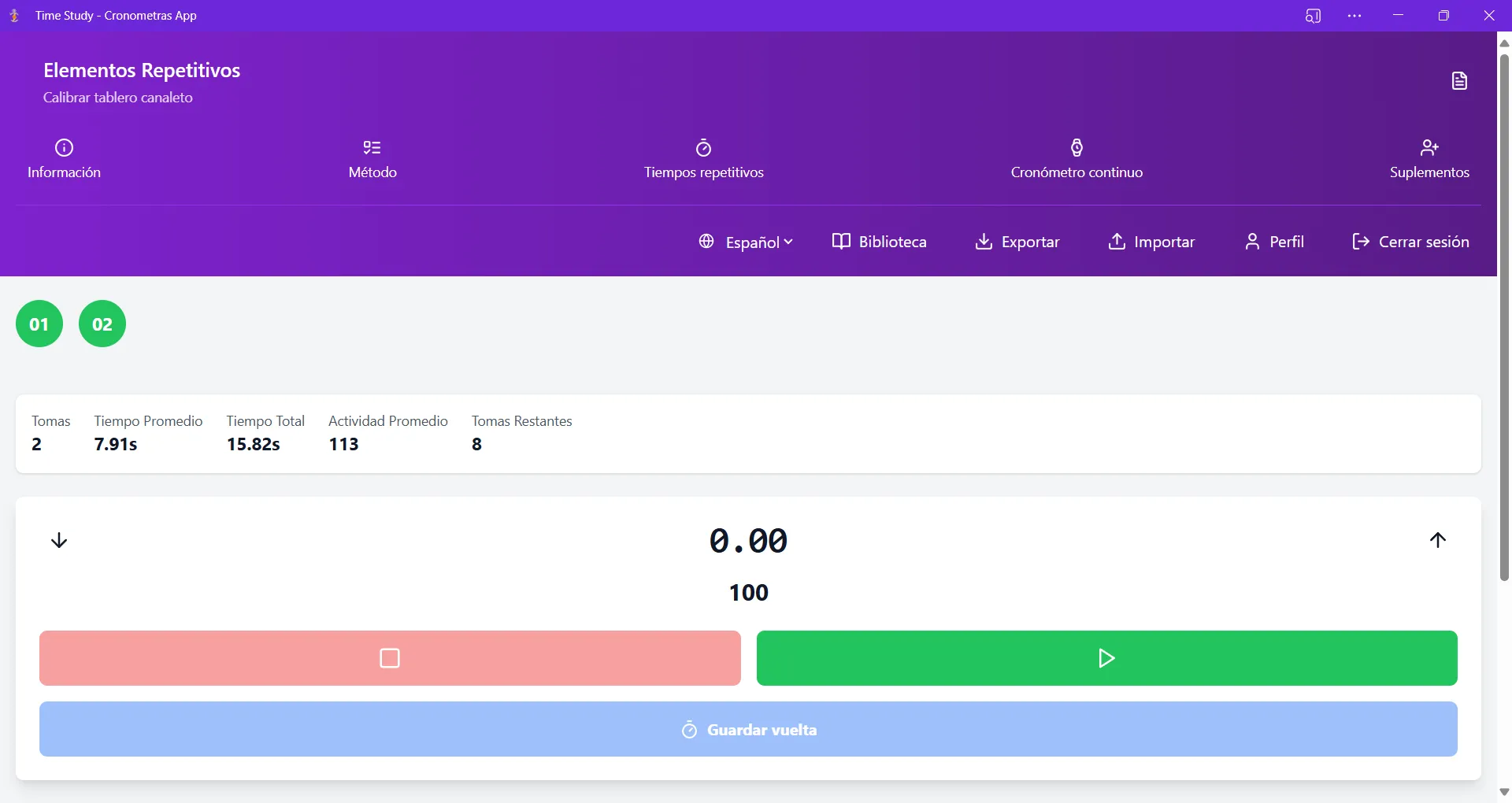
The Excel export functionality of CronometrasApp makes this analysis easier, allowing you to apply SPC formulas to the exported data or to visualize it directly in the platform.
Process Capability Analysis ($C_p$ and $C_{pk}$)
In the context of time study, capability analysis tells us whether our process can consistently meet the target time ($T_{obj}$). The indices are:
Potential Capability Index ($C_p$)
Where is the upper specification limit and the lower specification limit. A is considered adequate.
Actual Capability Index ($C_{pk}$)
It also considers the centering of the process:
Practical interpretation: If for a welding operation we have seconds with a tolerance of ±10% (LIE=54, LSE=66), and :
A of 0.53 indicates that the process is not capable of consistently meeting the specification, and the main cause is the off-centering (it is skewed toward the LIE). This tells us that we must retrain the operator or review the method before continuing to measure.
Identifying Causes of Variation: Ishikawa Diagram for Time Study
The cause-and-effect diagram (fishbone) helps us categorize the sources of variability into six classic dimensions (the 6Ms):
- Manpower: training level, fatigue, motivation, turnover
- Machine: maintenance condition, wear, calibration, actual vs nominal speed
- Material: dimensional variability, hardness, moisture, supplier defects
- Method: sequence of operations, tools, workplace ergonomics
- Measurement: stopwatch accuracy, start/finish criteria, analyst bias
- Environment: temperature, lighting, noise, humidity
For each source identified, SPC allows us to quantify its contribution by means of variance component studies or random-effects ANOVA.
Practical Case: Variability Reduction in a Packaging Line
Let us look at a real case. A pharmaceutical plant had capacity problems on its blister packaging line. The nominal cycle time was 12 seconds per blister, but actual output varied enormously.
Phase 1 — Initial sampling: 120 cycles were timed (20 subgroups of 6) across three shifts. Results: s, s, .
Phase 2 — Control charts: The mean chart revealed three points outside the upper limit, all during the night shift. The range chart showed an increasing pattern toward the end of each shift.
Phase 3 — Causal analysis: The Ishikawa diagram pointed to two main causes: (a) the thermoforming machine lost temperature after 6 hours of continuous operation, and (b) the night shift operator had only 3 weeks of experience.
Phase 4 — Corrective actions: Preventive maintenance every 4 hours (temperature recalibration) was implemented and a mentor was assigned to the night operator. After two weeks, the study was repeated: s, s, . The went from 0.62 to 1.41.
Result: Line capacity increased by 18% without capital investment, simply by applying SPC to understand and reduce variability.
Software for SPC in Time Study: How to Choose
Although Excel remains the most widely used tool for basic SPC analysis, specialized solutions exist:
- Minitab: the de facto standard for industrial SPC, with step-by-step wizards for control charts and capability analysis
- CronometrasApp: integration of digital time study with export of structured data ready for SPC analysis, allowing you to record times accurately and export them directly to Excel to build your charts
- JMP (SAS): advanced statistical analysis with integrated design of experiments capabilities
- R + qcc/SixSigma packages: open-source alternative for analysts with programming knowledge
The advantage of CronometrasApp in this ecosystem is that it solves the data capture problem, the most tedious part of SPC. With its digital stopwatch, voice entry and organization by elements, you get clean, structured data that you only have to import into your preferred statistical tool.
Common Mistakes When Applying SPC in Time Study
Confusing common-cause variation with special-cause variation: 85% of quality problems have common (systemic) causes. Adjusting the process when it is not warranted (overcontrol) increases variability.
Insufficient sample size: calculating or with fewer than 100 observations produces very imprecise estimates.
Ignoring autocorrelation: in continuous processes, consecutive observations are not independent. Standard control charts assume independence; if this is not met, EWMA or CUSUM charts must be used.
Not stratifying the data: mixing different shifts, machines or operators in a single analysis hides important patterns.
Using only the mean: as we saw at the beginning, the mean without measures of dispersion is misleading. Always accompany the mean with , and .
Conclusions
Modern industrial time study cannot be limited to pressing a button and writing down numbers. Variability is a reality in any production process, and Statistical Process Control provides us with the tools to understand, measure and reduce it systematically.
Integrating SPC into your time studies will allow you to:
- Establish standard times based on data, not on intuitions
- Distinguish between method problems and execution problems
- Justify improvement investments with quantitative evidence
- Monitor process stability over time
With tools like CronometrasApp for accurate data capture and software like Minitab or R for statistical analysis, any methods engineer can apply these techniques without needing to be an expert statistician.
Request a Cronometras Demo and discover how our digital time study platform helps you capture structured data ready for SPC analysis, with direct export to Excel, customizable element libraries and real-time collaboration for your methods engineering team.
Don't want to do it yourself? We do it for you from €800
If you prefer to outsource it, Cronometras delivers a complete time and motion study from a single video: elemental breakdown, OIT/TAL fatigue allowances, standard time with tolerances, and a report in PDF + Excel + JSON ready to present to management.