The 2025 Reality: If your engineering department still calculates machine assignment based on the classic deterministic model ($Cycle = Max(Man, Machine)$), your production standards are, with high probability, overestimated between 5% and 15%.
In plants with high automation or flexible manufacturing cells, variability is not an exception, it is the norm. The true challenge for the Plant Engineer today is not achieving theoretical Mechanical Saturation, but optimizing Expected Total Cost (ETC) by managing system stochasticity.
From the Engineering Division of Cronometras, we present this technical guide on the transition from static diagram to dynamic modeling, integrating Ashcroft interference tables and new cognitive ergonomics requirements from ISO 10075 standard.
Technical Fundamentals of Combined Cycle (Critical Variables)
To standardize technical language and avoid ambiguity in time studies, it is imperative to define variables with mathematical rigor before applying any assignment algorithm.
Time Breakdown ($TE, TI, TT$)
Correct segregation of times is the first step for system viability:
- External Time ($TE$): Comprises all manual activity that the operator must mandatorily perform with the machine stopped (e.g., loading/unloading, part centering).
- Technical Note: Reducing is the main objective of SMED methodologies. High directly penalizes machine availability.
- Internal Time ($TI$): Manual activity performed by the operator while the machine is in automatic cycle (e.g., deburring, dimensional inspection, packaging). This time is "free" from the machine cycle perspective, provided .
- Technological Time ($TT$): Automatic process time.
- Common Error: Considering as an absolute constant. In CNC machining or plastic injection processes, variables like material hardness or temperature can introduce variations. For H-M calculation, standard deviation ($\sigma) of $TT must be used for robust models.
Theoretical Assignment Formula ($N$)
The theoretical number of machines ($N$) an operator can attend is defined by the relationship between total cycle and dedication time per machine:
The integer number dilemma: The result of is rarely an integer. The engineer faces a binary decision with financial consequences:
- Option (lower integer): The operator has wait times (low saturation). Machines never wait for the operator. Production per machine is maximized.
- Option (upper integer): The operator is over-saturated. Machines wait for attention (interference). Labor productivity is maximized, but OEE per machine drops.
The Error of Determinism: Machine Interference Calculation
Here lies the "Pain Point" of most traditional industrial timing. By assuming cycles are perfectly synchronized "Swiss clocks", Machine Interference ($I$) is ignored.
From Theory to Stochastic Reality
Interference occurs when one or more machines stop (end of cycle or random stop) while the operator is busy attending another machine. In a deterministic system, this is "drawn" so it doesn't happen. In stochastic reality, system entropy generates waiting queues.
Ignoring random interference and desynchronization reduces real production regarding theoretical, invalidating production incentives and standard cost calculation.
Application of Ashcroft Tables and Wright Formulas
To calculate time lost due to interference in systems of machines attended by one server, we must resort to probabilistic models (M/M/1 or M/M/c Queuing Theory).
- Ashcroft Tables: Use Service Coefficient ($ \rho = \frac{TE+TI}{TT} $) and number of machines ($n$) to return average expected interference percentage.
- Example: An operator with 4 machines and a 20% service coefficient does not have 0% interference (as simple arithmetic would say), but statistically close to 12.4% according to Ashcroft tables, due to stop coincidence probability.
- Wright Formulas: Recommended when machine cycle times are significantly different from each other.
Regulatory Framework Spain 2025: Cognitive Ergonomics and Safety
Methods engineering in 2025 must not only respond to productivity, but to strict legal compliance. Cronometras authority is based on integrating ILO and ISO regulations into technical calculation.
ISO 10075 and Mental Load in Multi-Machine Tasks
Labor Inspection is shifting focus towards psychosocial load. An H-M diagram saturating the operator at 98% is technically viable on paper, but illegal and unsustainable in practice under UNE-EN ISO 10075 (Ergonomic principles related to mental workload).
- Divided Attention Fatigue: Managing multiple asynchronous processes raises cognitive fatigue.
- The 85% Limit: At Cronometras, we recommend establishing an active saturation limit of 85%. The remaining 15% is not "leisure", it is a buffer for cognitive recovery and management of non-tabulated micro-incidents.
- ILO Allowances ($K$): Rest coefficients must be recalculated penalizing multiple surveillance of high-risk or high-precision processes.
Interaction Safety (Industry 4.0)
Safety integration in the standard cycle is non-negotiable. times must include safety protocols.
- Digital LOTO: If the machine requires safe stops for loading/unloading, lock-out/tag-out time (software or hardware) is part of the Standard Cycle, not unproductive time. Ignoring it causes safety violations due to time pressure.
Cronometras Methodology: Economic vs. Technical Optimization
How do we decide final assignment? The answer is not technical, it is financial.
Minimum Unit Cost Criterion
The goal is to minimize cost per piece produced, not necessarily maximize gross production. The decision formula we propose to plant management is:
Sensitivity Analysis:
- If Machine Hourly Cost is high (e.g., 5-axis Machining Centers), the strategy must be minimizing machine interference (assign low , operator with wait times).
- If Labor Cost is the main driver (simple processes, amortized machines), the strategy is saturating the operator (assign high , assuming machine stops).
Time Standardization with MOST and MTM
"Snapback" timing is inefficient for designing multi-machine cells. Predicting time before physical implementation is required.
- The "Walking Time" factor: In H-M diagrams, displacement between machines is the most critical and volatile variable.
- Use of Basic MOST: We use Maynard Operation Sequence Technique to simulate different layouts. MOST allows us to calculate with precision the impact of changing machine arrangement (reducing meters traveled) without moving a single piece of equipment, validating cycle feasibility.
Practical Implementation: From Excel to MES (Digital Twin)
Concurrency Time Audit
The first step is auditing current standards. Many ERPs contain routes with times calculated years ago under deterministic premises. It is vital to recalculate installed capacity applying Ashcroft interference factors to obtain realistic Capacity Planning.
Integration with MES Systems
The H-M diagram must not be a static document. It must feed from the MES (Manufacturing Execution System). By capturing real micro-stops and real-time cycle variability, we can dynamically adjust the number of machines assigned per shift, creating a dynamic and adaptive OEE.
Conclusions for Engineering Management
Machine assignment in 2025 demands abandoning arithmetic simplicity in favor of statistical modeling and regulatory compliance. The three pillars for successful implementation are:
- Interference Modeling: Mandatory use of Ashcroft Tables or queue simulation to predict real OEE loss.
- Cognitive Limit: Respecting the 85% saturation ceiling (ISO 10075) to guarantee quality and sustainable safety.
- Rigorous Standardization: Use of MOST/MTM standards to fix manual and walking times, eliminating direct timing subjectivity.
Do your time standards ignore machine interference or cognitive load? The difference between theoretical and real production is lost money. Request a technical saturation and methods audit with the Engineering Division of Cronometras.
Article developed by the Cronometras technical team – Specialists in Methods and Time Engineering.