Introduction
In every industrial operation, there is a phenomenon as predictable as it is undervalued: operators get faster with practice. What initially takes 10 minutes can drop to 6 after a hundred repetitions. This reality, formalized mathematically as the learning curve, has profound implications for anyone who calculates standard times.
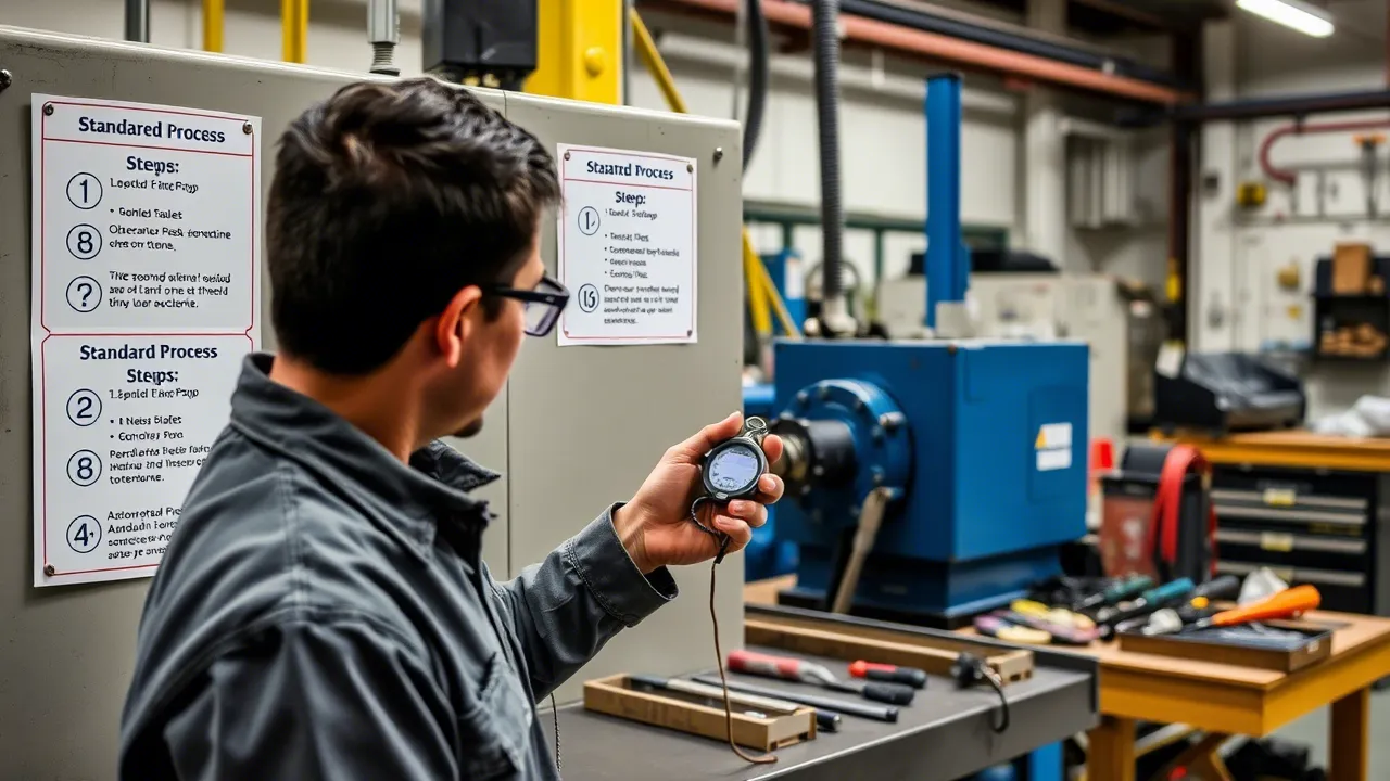
Imagine an assembly line that has just launched a new product. The time study analyst visits on the first day, times the operations, and establishes a standard time. Three weeks later, that standard is already obsolete: the operators have developed skill, eliminated micro-pauses, and found shortcuts that reduce the actual time by 25%.
Should the time study ignore this effect or incorporate it? The answer, backed by decades of industrial engineering, is clear: the learning curve is not an anomaly to be dismissed, but a fundamental parameter of standard setting. In this article we explore its mathematical formulation, its application to industrial time study, and how digital tools such as CronometrasApp make it easier to manage.
What Is the Learning Curve?
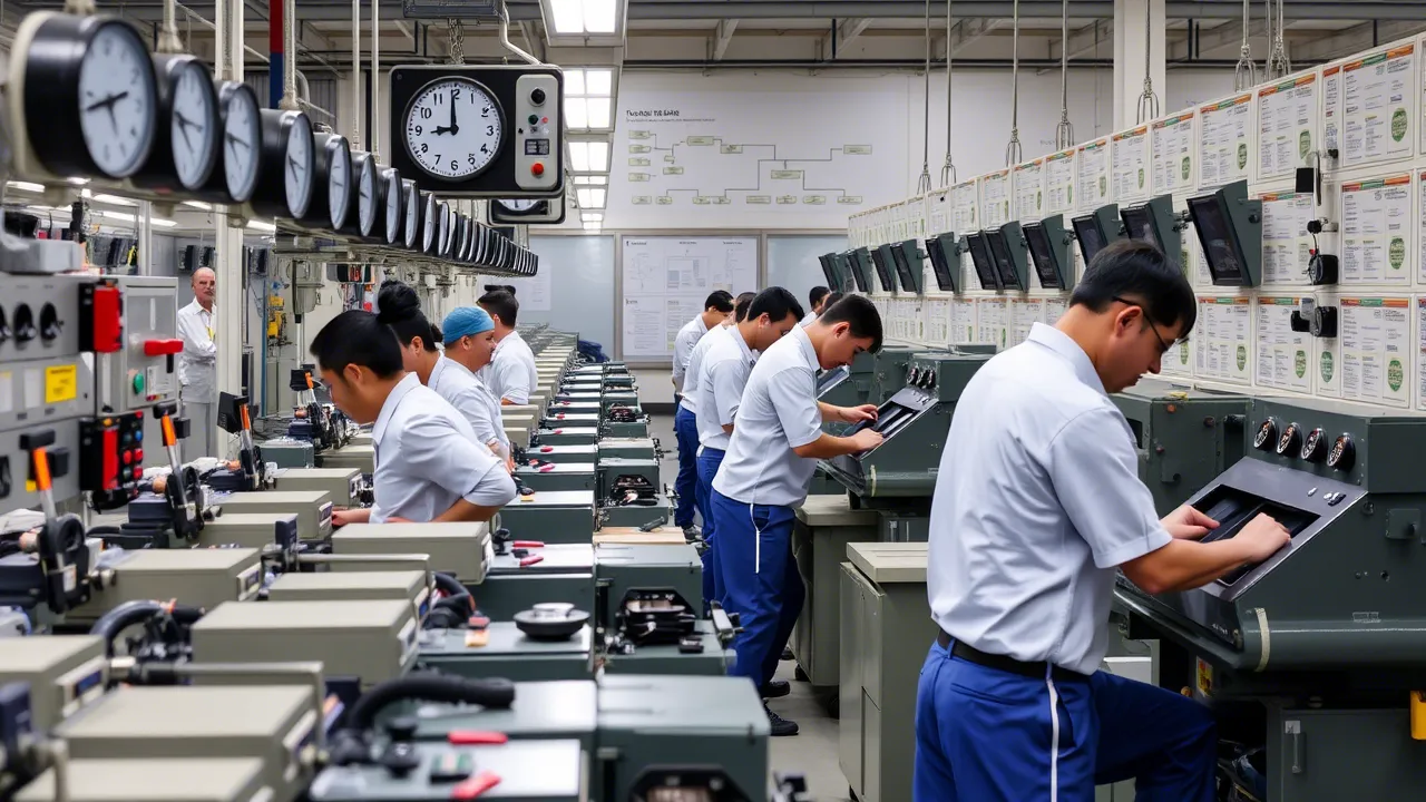
The learning curve —or learning curve— describes the relationship between the cumulative number of units produced and the time required to produce each additional unit. It was first observed in 1936 by T.P. Wright in the aircraft industry, who documented that aircraft assembly time decreased by a constant percentage every time cumulative production doubled.
The Universal Constant
The principle is simple: every time cumulative production doubles, the time per unit decreases by a fixed percentage, called the learning rate ($L$). Typical values range from 70% to 95%:
- 80% rate: when production doubles, the time per unit drops to 80% of the previous one. Typical of complex manual assembly.
- 90% rate: a more modest reduction. Common in semi-automated operations.
- 95% rate: an almost flat curve. Highly mechanized operations where the human factor is minimal.
The lower the percentage, the steeper the curve: 70% represents very rapid learning (typical of consumer electronics), while 95% indicates that the operation is already close to its efficiency limit.
Wright's Formula
The classic mathematical formulation of the learning curve is:
Where:
- = Time to produce the n-th unit
- = Time to produce the first unit
- = Cumulative unit number
- = Learning exponent, calculated as:
Where is the learning rate expressed as a decimal (for example, 0.80 for an 80% rate).
Practical Example
Suppose the first unit of an electronic assembly requires minutes, and a learning rate of 85% is estimated ($L = 0.85$). How long will unit number 20 take?
Step 1 — Calculate the exponent :
Step 2 — Apply Wright's formula:
In just 20 units, the time has been cut in half. And for unit 100:
Total Cumulative Time
To plan workloads and costs, we need the cumulative time to produce the first units:
Or using the integral approximation (accurate enough for $n > 10$):
In our example, the total time for 100 units would be approximately:
Implications for Time Study
The learning curve poses a methodological dilemma for the time study analyst. If an operation is timed in its early phase, the resulting standard will be generous in the long run. If you wait for stabilization, the standard will be unattainable during the ramp-up phase.
When to Incorporate the Learning Curve
The decision to include the learning curve in the standard or not depends on the production context:
| Scenario | Incorporate curve? | Justification |
|---|---|---|
| Stable mass production (>10,000 units) | No | The effect is diluted. The stabilized time is the relevant one. |
| Small batches (<500 units) | Yes | Learning dominates the entire batch. Fixed standard = cost overrun. |
| New product launch | Yes (ramp-up) | Tiered standard: month 1, month 2, month 3 with decreasing targets. |
| High personnel turnover | Yes | Every new operator goes through the curve. The standard must reflect the team average. |
| Highly automated operation | No | The machine does not learn. The human factor is residual. |
Dynamic Standard Time
One advanced practice, made easier by digital tools such as CronometrasApp, is to establish dynamic standard times that adjust automatically according to the cumulative volume produced. The system can apply Wright's formula in real time, generating realistic targets for each phase of the product life cycle.
Determining the Learning Rate ($L$)
Where does the value of come from? There are several methods:
1. Historical Data from Similar Products
The most reliable source. If the company manufactured an analogous product, is calculated from the recorded times:
Or more practically, using the slope of the regression line on a log-log scale:
Plotting against , the slope of the line is , and from there .
2. Estimation by Type of Operation
When there is no historical data, indicative tables based on the nature of the task are used:
- Fine electronic assembly: 70-75%
- Manual mechanical assembly: 75-85%
- Manual welding: 80-85%
- CNC machining (loading/unloading): 85-90%
- Visual inspection processes: 80-88%
- Warehouse operations (picking): 82-90%
- Manual packing: 78-85%
3. Two-Point Method
If the first units have been timed, can be estimated with just two points:
Where and are the times of the first and the k-th unit, respectively. This method is more reliable if , since the first units show high variability.
Practical Applications in Industry
Case 1: Planning a New Production Batch
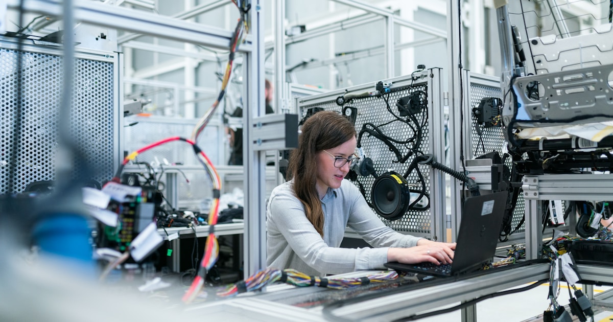
An electrical harness factory receives an order for 500 units of a new design. Methods engineering calculates minutes and estimates .
- Unit 500: min
- Total batch time: approximately 4,700 minutes (78.3 hours)
If a fixed standard of 18 minutes were used, minutes (150 hours) would be budgeted. The difference is a 48% overestimation that inflates costs and lead times and discourages improvement.
Case 2: Calculating the Break-Even Point for Automation
A company is evaluating whether to automate an assembly station. The machine has a fixed time of 4 minutes per unit but requires an investment of 80,000 €. Manual assembly starts from min with .
From what volume is automation profitable?
Cumulative manual time for units (integral approximation):
The labor cost is 22 €/hour. The machine pays for itself in 3 years. The break-even point is reached when the labor savings equal the cost of the machine. Solving numerically, with approximately 12,000 units per year, automation is justified from the second year onward.
Case 3: Performance Evaluation with the Learning Curve
A common mistake in factory environments is to evaluate new operators against the standard time of the veterans. An operator in their first week with an 80% learning rate may be performing at half the standard speed... and not for lack of capability, but because they are climbing their own curve.
Learning-curve-based management makes it possible to set progressive targets that motivate without demoralizing:
| Week | Cumulative units | Expected time (min) | Reasonable target |
|---|---|---|---|
| 1 | 50 | 7.8 | 8.5 (-10% slack) |
| 2 | 150 | 5.9 | 6.5 |
| 3 | 300 | 5.0 | 5.5 |
| 4 | 500 | 4.4 | 4.8 (approx. to standard) |
Learning Curve in CronometrasApp
Modern digital tools have transformed learning-curve management from an academic exercise into an operational reality. CronometrasApp includes features that allow the time study analyst to:
Automatic chronological logging: each timed cycle is linked to the operator and the unit number produced, building the database needed to fit the curve.
Customizable element libraries: standard times by category can be segmented by learning phase (learning, competent, expert), making it easier to assign differentiated targets.
Integrated OIT allowances analysis: fatigue allowances can be adjusted during the learning phase, where the cognitive effort is greater and fatigue appears earlier.
Export to Excel: time data per cumulative unit can be exported for external regression analysis and calculation of and using statistical tools.
Real-time collaboration: supervisors and analysts share the same data view, easing the transition from temporary standards to definitive standards.
Common Mistakes When Applying the Learning Curve
1. Confusing Correlation with Causation
The fact that times go down does not mean it is due to learning. It may be caused by material improvements, machine adjustments, or subtle changes in the method. Wright's curve measures organizational learning, not just individual learning. The analyst must document whether the observed changes stem from operator skill or from modifications external to the process.
2. Ignoring Interruptions
If production stops for weeks (vacations, batch change, breakdown), the phenomenon of forgetting or forgetting curve occurs. Wright's formula does not account for this. For intermittent batches, a retention factor must be applied that artificially increases the estimated time:
Where is the number of interruption days and is the daily forgetting factor (typically 0.001-0.005).
3. Using the Same Rate for the Entire Product Life
The learning rate is not constant. In very early phases it may be 70%, stabilizing at 90-95% once the productivity plateau is reached. A recommended practice is to use segmented curves: one rate for the first 100 units, another for the next 400, and a fixed time from unit 500 onward.
Conclusion
The learning curve is not a theoretical concept reserved for textbooks. It is an operational reality that, when properly managed, saves millions in labor costs, improves the accuracy of planning, and humanizes performance evaluation by recognizing that every operator needs time to reach their full potential.
Ignoring it leads to inflated standards that hide inefficiency, or to impossible standards that burn out teams. Incorporating it rigorously — supported by tools such as CronometrasApp for data logging and analysis — turns time study into a predictive discipline, not just a descriptive one.
The next time you walk through your plant and see a new operator, remember: they are writing their own learning curve. And the job of the time study analyst is to make sure that curve has the right slope.
Don't want to do it yourself? We do it for you from €800
If you prefer to outsource it, Cronometras delivers a complete time and motion study from a single video: elemental breakdown, OIT/TAL fatigue allowances, standard time with tolerances, and a report in PDF + Excel + JSON ready to present to management.